Credits: Forked from deep-learning-keras-tensorflow by Valerio Maggio
Unsupervised learning
AutoEncoders
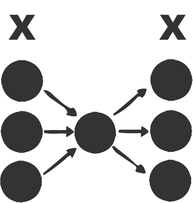
An autoencoder, is an artificial neural network used for learning efficient codings.
The aim of an autoencoder is to learn a representation (encoding) for a set of data, typically for the purpose of dimensionality reduction.
Unsupervised learning is a type of machine learning algorithm used to draw inferences from datasets consisting of input data without labeled responses. The most common unsupervised learning method is cluster analysis, which is used for exploratory data analysis to find hidden patterns or grouping in data.
# based on: https://blog.keras.io/building-autoencoders-in-keras.html

encoding_dim = 32
input_img = Input(shape=(784,))
encoded = Dense(encoding_dim, activation='relu')(input_img)
decoded = Dense(784, activation='sigmoid')(encoded)
autoencoder = Model(input=input_img, output=decoded)
encoder = Model(input=input_img, output=encoded)

encoded_input = Input(shape=(encoding_dim,))
decoder_layer = autoencoder.layers[-1]
decoder = Model(input=encoded_input, output=decoder_layer(encoded_input))

autoencoder.compile(optimizer='adadelta', loss='binary_crossentropy')

(x_train, _), (x_test, _) = mnist.load_data()

x_train = x_train.astype('float32') / 255.
x_test = x_test.astype('float32') / 255.
x_train = x_train.reshape((len(x_train), np.prod(x_train.shape[1:])))
x_test = x_test.reshape((len(x_test), np.prod(x_test.shape[1:])))

#note: x_train, x_train :)
autoencoder.fit(x_train, x_train,
                nb_epoch=50,
                batch_size=256,
                shuffle=True,
                validation_data=(x_test, x_test))
Testing the Autoencoder
encoded_imgs = encoder.predict(x_test)
decoded_imgs = decoder.predict(encoded_imgs)

n = 10
plt.figure(figsize=(20, 4))
for i in range(n):
    # original
    ax = plt.subplot(2, n, i + 1)
    plt.imshow(x_test[i].reshape(28, 28))
    plt.gray()
    ax.get_xaxis().set_visible(False)
    ax.get_yaxis().set_visible(False)

    # reconstruction
    ax = plt.subplot(2, n, i + 1 + n)
    plt.imshow(decoded_imgs[i].reshape(28, 28))
    plt.gray()
    ax.get_xaxis().set_visible(False)
    ax.get_yaxis().set_visible(False)
plt.show()
Sample generation with Autoencoder
encoded_imgs = np.random.rand(10,32)
decoded_imgs = decoder.predict(encoded_imgs)

n = 10
plt.figure(figsize=(20, 4))
for i in range(n):
    # generation
    ax = plt.subplot(2, n, i + 1 + n)
    plt.imshow(decoded_imgs[i].reshape(28, 28))
    plt.gray()
    ax.get_xaxis().set_visible(False)
    ax.get_yaxis().set_visible(False)
plt.show()
Pretraining encoders
One of the powerful tools of auto-encoders is using the encoder to generate meaningful representation from the feature vectors.
# Use the encoder to pretrain a classifier
Natural Language Processing using Artificial Neural Networks
“In God we trust. All others must bring data.” – W. Edwards Deming, statistician
Word Embeddings
What?
Convert words to vectors in a high dimensional space. Each dimension denotes an aspect like gender, type of object / word.
“Word embeddings” are a family of natural language processing techniques aiming at mapping semantic meaning into a geometric space. This is done by associating a numeric vector to every word in a dictionary, such that the distance (e.g. L2 distance or more commonly cosine distance) between any two vectors would capture part of the semantic relationship between the two associated words. The geometric space formed by these vectors is called an embedding space.
Why?
By converting words to vectors we build relations between words. More similar the words in a dimension, more closer their scores are.
Example
W(green) = (1.2, 0.98, 0.05, …)
W(red) = (1.1, 0.2, 0.5, …)
Here the vector values of green and red are very similar in one dimension because they both are colours. The value for second dimension is very different because red might be depicting something negative in the training data while green is used for positiveness.
By vectorizing we are indirectly building different kind of relations between words.
Example of word2vec using gensim
from gensim.models import word2vec
from gensim.models.word2vec import Word2Vec
Reading blog post from data directory
import os
import pickle
DATA_DIRECTORY = os.path.join(os.path.abspath(os.path.curdir), 'data')
male_posts = []
female_post = []
with open(os.path.join(DATA_DIRECTORY,"male_blog_list.txt"),"rb") as male_file:
    male_posts= pickle.load(male_file)

with open(os.path.join(DATA_DIRECTORY,"female_blog_list.txt"),"rb") as female_file:
    female_posts = pickle.load(female_file)
print(len(female_posts))
print(len(male_posts))
filtered_male_posts = list(filter(lambda p: len(p) > 0, male_posts))
filtered_female_posts = list(filter(lambda p: len(p) > 0, female_posts))
posts = filtered_female_posts + filtered_male_posts
print(len(filtered_female_posts), len(filtered_male_posts), len(posts))
Word2Vec
w2v = Word2Vec(size=200, min_count=1)
w2v.build_vocab(map(lambda x: x.split(), posts[:100]), )
w2v.vocab
w2v.similarity('I', 'My')
print(posts[5])
w2v.similarity('ring', 'husband')
w2v.similarity('ring', 'housewife')
w2v.similarity('women', 'housewife') # Diversity friendly
Doc2Vec
The same technique of word2vec is extrapolated to documents. Here, we do everything done in word2vec + we vectorize the documents too
import numpy as np
# 0 for male, 1 for female
y_posts = np.concatenate((np.zeros(len(filtered_male_posts)),
                          np.ones(len(filtered_female_posts))))
len(y_posts)
Convolutional Neural Networks for Sentence Classification
Train convolutional network for sentiment analysis. Based on “Convolutional Neural Networks for Sentence Classification” by Yoon Kim http://arxiv.org/pdf/1408.5882v2.pdf
For ‘CNN-non-static’ gets to 82.1% after 61 epochs with following settings:
embedding_dim = 20
filter_sizes = (3, 4)
num_filters = 3
dropout_prob = (0.7, 0.8)
hidden_dims = 100
For ‘CNN-rand’ gets to 78-79% after 7-8 epochs with following settings:
embedding_dim = 20
filter_sizes = (3, 4)
num_filters = 150
dropout_prob = (0.25, 0.5)
hidden_dims = 150
For ‘CNN-static’ gets to 75.4% after 7 epochs with following settings:
embedding_dim = 100
filter_sizes = (3, 4)
num_filters = 150
dropout_prob = (0.25, 0.5)
hidden_dims = 150
it turns out that such a small data set as “Movie reviews with one sentence per review” (Pang and Lee, 2005) requires much smaller network than the one introduced in the original article:
embedding dimension is only 20 (instead of 300; ‘CNN-static’ still requires ~100)
2 filter sizes (instead of 3)
higher dropout probabilities and
3 filters per filter size is enough for ‘CNN-non-static’ (instead of 100)
embedding initialization does not require prebuilt Google Word2Vec data. Training Word2Vec on the same “Movie reviews” data set is enough to achieve performance reported in the article (81.6%)
** Another distinct difference is slidind MaxPooling window of length=2 instead of MaxPooling over whole feature map as in the article
import numpy as np
import data_helpers
from w2v import train_word2vec

from keras.models import Sequential, Model
from keras.layers import (Activation, Dense, Dropout, Embedding,
                          Flatten, Input, Merge,
                          Convolution1D, MaxPooling1D)

np.random.seed(2)
Parameters
Model Variations. See Kim Yoon’s Convolutional Neural Networks for Sentence Classification, Section 3 for detail.
model_variation = 'CNN-rand'  #  CNN-rand | CNN-non-static | CNN-static
print('Model variation is %s' % model_variation)
# Model Hyperparameters
sequence_length = 56
embedding_dim = 20
filter_sizes = (3, 4)
num_filters = 150
dropout_prob = (0.25, 0.5)
hidden_dims = 150
# Training parameters
batch_size = 32
num_epochs = 100
val_split = 0.1
# Word2Vec parameters, see train_word2vec
min_word_count = 1  # Minimum word count
context = 10        # Context window size
Data Preparation
# Load data
print("Loading data...")
x, y, vocabulary, vocabulary_inv = data_helpers.load_data()

if model_variation=='CNN-non-static' or model_variation=='CNN-static':
    embedding_weights = train_word2vec(x, vocabulary_inv,
                                       embedding_dim, min_word_count,
                                       context)
    if model_variation=='CNN-static':
        x = embedding_weights[0][x]
elif model_variation=='CNN-rand':
    embedding_weights = None
else:
    raise ValueError('Unknown model variation')
# Shuffle data
shuffle_indices = np.random.permutation(np.arange(len(y)))
x_shuffled = x[shuffle_indices]
y_shuffled = y[shuffle_indices].argmax(axis=1)
print("Vocabulary Size: {:d}".format(len(vocabulary)))
Building CNN Model
graph_in = Input(shape=(sequence_length, embedding_dim))
convs = []
for fsz in filter_sizes:
    conv = Convolution1D(nb_filter=num_filters,
                         filter_length=fsz,
                         border_mode='valid',
                         activation='relu',
                         subsample_length=1)(graph_in)
    pool = MaxPooling1D(pool_length=2)(conv)
    flatten = Flatten()(pool)
    convs.append(flatten)

if len(filter_sizes)>1:
    out = Merge(mode='concat')(convs)
else:
    out = convs[0]

graph = Model(input=graph_in, output=out)

# main sequential model
model = Sequential()
if not model_variation=='CNN-static':
    model.add(Embedding(len(vocabulary), embedding_dim, input_length=sequence_length,
                        weights=embedding_weights))
model.add(Dropout(dropout_prob[0], input_shape=(sequence_length, embedding_dim)))
model.add(graph)
model.add(Dense(hidden_dims))
model.add(Dropout(dropout_prob[1]))
model.add(Activation('relu'))
model.add(Dense(1))
model.add(Activation('sigmoid'))
model.compile(loss='binary_crossentropy', optimizer='rmsprop',
              metrics=['accuracy'])

# Training model
# ==================================================
model.fit(x_shuffled, y_shuffled, batch_size=batch_size,
          nb_epoch=num_epochs, validation_split=val_split, verbose=2)
Another Example
Using Keras + GloVe - Global Vectors for Word Representation
Using pre-trained word embeddings in a Keras model
Reference: https://blog.keras.io/using-pre-trained-word-embeddings-in-a-keras-model.html